Applying and interpreting staleness metric (Advanced dependency management - part 3)

If you have been following this series from the beginning, you are getting the appreciation why this seemingly simple problem hasn't been solved yet. In Part 1, I described the background and motivation, and in Part 2, I discussed the details of the operations that need to be performed during integration and introduced a robust staleness metric. As a reminder, we're working with this graph of module dependencies, with 200 modules, and 12 levels in depth. Each vertex represents a module, and each edge represents a dependency.

First, we compute Dependency Graph Staleness Metric, DGSM, introduced previously. We find out, that the value is 19,733. That number by itself gives us some idea as to the amount of integration that needs to be performed, since we can interpret each point in the metric as incrementing a single dependency between two modules and running the build to verify that the downstream module is compatible with the new version. Note that there will always be certain staleness in the graph, since even in a most aggressively integrated system, there will always be changes that are in the process of being propagated. But what constitutes a healthy amount of staleness?

Obtaining day-by-day historical data would be time consuming, but we can get some perspective on how far out of this ideal state our system is by looking at the extremes of the metric. One way would be to calculate the metric for each module being one version behind. A graph with this property has DGSM value of 5,015. So we can also say on average the modules in the current graph are 4 versions behind. This tells us a bit how the structure of this graph impacts the metric, but as we will soon find out, majority of the modules in the graph have less than 4 versions.

A better way to look at the staleness would be to estimate the total amount of integration performed on the graph since its inception. We can do this by assuming all dependencies were pointing at the oldest versions. The DGSM metric in that case would be 73,246. This is a good approximation of the total cost of integration that the system has incurred. This graph of jars was converted to a new build system 2 years ago, at which point all dependencies were set to the latest and the value of the metric would have been 0. From that, we can compute monthly staleness attrition, which is about 3,000. One way to interpret the current staleness, at almost 20,000 is to say that the system is between 6 and 7 months behind.

These findings are summarized in the table below.

Current DGSM	19,733
Each module one version behind	5,015
Monthly attrition	3,000
Historic total (2 yrs.)	73,246

Despite the tedious cost of manual integration, this graph has been somewhat kept up to date over time. 75% of the integration work has been performed by developers, leaving the graph 25% stale (current 19,733 divided by historic total 73,246). Since individual developers never had the insight into staleness we are getting right now, we can conclude that this relatively high rate of integration was the minimum necessary to deliver code into production. Continuous Integration is organically occurring in this graph.

Talk at the 2015 Strange Loop

The previous two posts were a teaser for my talk at Strange Loop, where I took these ideas and applied them to my dataset. Over the next few weeks, I will be discussing in detail the material in the talk, and going more in depth in some places. For now, I wanted to give quick thanks to the organizers for having this talk, and to the audience for the active participation and lively discussion at the end of a 12 hour day. I got many good suggestions, and equally importantly, nobody got up and said "hey it's a solved problem, why don't you just read X and use Y." This reassures me that Dependency Integration is a direction worth pursuing.

Here is the slide deck from the talk. (In my talks, slides are just props for spoken word, and so I wouldn't be surprised if they were confusing without context.)

Measuring staleness (Advanced dependency management - part 2)

Dependency management at scale

This is part 2 of a series of posts documenting my attempts at understanding and writing software to support dependency management. In order to limit the scope, the first problem I wanted to solve is keeping Java module dependencies up to date. In previous post I introduced the problem and gave a bit of background on the way versioned jar dependencies work. In this post, we will explore the a real versioned module ecosystem and come up with a way to keep it up to date.

Jez Humble's Continuous Delivery book discusses dependency management on a simple example.

The example I got to work with, is the graph of versioned Java libraries at my company, which looks like this: In the above graph, red edges indicate out of date, stale, dependencies, red circles indicate modules which do not build (due to failing tests or other reasons), and blue edges indicate presence of a cycle. As you can see, at scale, the dependency integration presents a new set of challenges.

Given a module ecosystem like the one above, is not possible to successfully update all dependencies in one pass. The modules whose builds are failing cannot be updated automatically, and they block any propagation of updates up the graph. Additionally, we can expect some updates to be incompatible, and cause more failures in upstream modules. Last, but not least, some critical issues may not be caught by the tests until much higher levels on the graph are reached, leading to entire subtrees being unreleasable and affecting release schedule of applications that depend on them.

Since it's not apparent to human eye that a small batch of version updates has improved the staleness of the graph, a staleness metric is necessary to show and chart progress. Additionally, from studying this metric over time, we can determine how it normally grows, and what is the happy spot for this ecosystem once we begin to reduce the staleness.

Naive metric

On the first attempt, one may construct a metric that simply measures the number of stale edges on the graph. The lower the number, the better (more integrated) the modules would be. However, there is a problem with this approach. Consider a simple case with one out of date dependency at the bottom rank of the graph (outdated dependency in red).

The initial staleness metric value is 1. Once we update this dependency, we need to publish a new artifact with updated dependency, and we find that the 3 downstream projects are now outdated. The value of the metric is 3.

So even though we reduced the staleness in the graph, the naive staleness metric just went up. Eventually, we would complete the integration, leaving all edges up to date, but keep in mind that we are operating in the environment where complete integration isn't possible and may not even be desirable. So a staleness metric we use needs to account accurately for partial improvements. Any update of a dependency in the graph should result in staleness metric reduction.

A better metric

A better metric simply takes into account the flaw described in previous metric - total cost of integration. In order to compute the value, we must know a position of a module in the graph, and consider all the steps necessary for complete integration. We take one stale dependency at a time and enumerate all the steps it would take to completely integrate that change. In other words, we count the number of edges in the spanning tree rooted at the module whose stale dependency is being updated. So, in the first picture above, the staleness metric would be 4, and after updating the first direct dependency, it would be 3. To get a better feel, let's look at some more complicated examples.

In the example below, there are two modules that have outdated dependencies. We are also beginning to address modules by name, which is determined by their rank in the graph and position within that rank.

Keep in mind that integration may fail, so we need to consider each of the outdated edges separately. We first calculate the dependency staleness for module "20", which is 3 (10, 20, 30, 31). We then calculate staleness for module 21, which is 2 (10, 21, 31). So the total staleness value is 5.

From this diamond dependency, a special case arises if diamond dependencies are present downstream. In the graph below, once we begin integration, module 20 is out of date, and by the same logic as we used above, the dependency between 40 and 50 should be counted twice, once when integration is coming from the left, once when it's coming from the right.

However, for the little value that it adds in some edge cases, this requirement adds too much complexity to calculating the metric, so I arbitrarily choose to ignore diamond dependencies if they are not directly involved in the stale edge that's being calculated. Therefore staleness metric for the graph in this example is 6 (and not 7).

We introduce versions

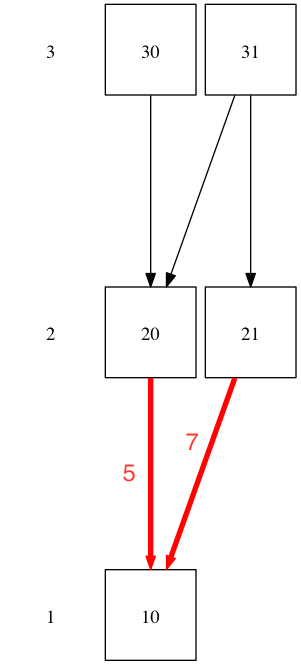
So far we considered the staleness of a single dependency staleness as binary - it's either stale or not. But to accurately reflect reality we need to take into account how many versions behind the given dependency is. The underlying principle is that the metric needs to take into account the smallest reductions in staleness, even if integration with the latest version isn't possible. Therefore, in calculating staleness, we should pretend that we're integrating each version separately. In practice, the calculation can be accomplished by multiplying the metric calculated for a stale edge by number of versions that that edge is behind. Consider the example below, where one dependency is 5 versions behind, and the other 7:

The staleness metric in the above example is 29 (3 x 5 + 2 x 7).

Next issue to consider, once we start looking at the past is that the dependency graph changes over time. (There's a visual example in the previous post.) For this metric, I propose to only consider the most recent version of the graph. There are two reasons for that - one is simplicity of computing the metric, another is that I don't want old dependencies unnecessarily weighing in on the staleness.

To better understand this latter reason, consider an extreme case of a jar which still has some old versions of other jars depend on it, but which no current version depends on. If we tried to improve the metric directly, we'd check out downstream modules, only to find out they no longer depend on the jar - so there would be nothing to do. Since we ignore past versions of the dependency graph, this jar's contribution to staleness metric is 0, and whoever is trying to improve the metric will not waste time trying to update a version of that jar.

At the end of this section, one final example, of multiple stale dependencies. Analyzing this example will give us a good insight into the strength of this metric.

First, let's calculate staleness as exercise. We consider each stale edge separately, and generate a spanning tree with that edge. So we have the following trees:
(20, 30) with staleness of 5
(20, 31) with staleness of 3
(10, 20, 30, 31) with staleness of 4
(10, 21, 31) with staleness of 2
The total is 24 (5 x 1 + 3 x 1 + 4 x 3 + 2 x 2).

If this seems a bit awkward, consider how you would approach integration if there were several toxic dependencies which would break downstream builds, and yet you still wanted to integrate as much as possible. If latest version of 20 broke in integration with 30, or 10's latest version broke 31, you would want to integrate as much as possible before things broke. So consider this partially integrated graph, where breaking changes above prevented further integration.

Let's look at how the edge between 20 and 30 got to be 5 versions behind. At first, we'd integrate as much as possible of 20 into 30 only to find out that the latest does not work. So at that point, the 20-30 edge would be one version behind. Then we might try and integrate 10 into 20 all the way, producing 4 more versions of 20, none of which could be integrated into 30, leaving the 20-30 edge 5 versions behind again. At that point, 20-31 would be 7 versions behind, but only latest version of 10 being toxic to 31, the integration could proceed all the way to the last-but-one version of 20, leaving the edge 20-31 one version behind. The same process would take place around the 10-21-31 tree.

Note that we did quite a bit of integration, and actually exposed backwards incompatible breaks in our code. We'd expect the integration metric to go down significantly, and indeed when we calculate it, we see that it is down from 24 only to 7.

Advanced dependency management - Part 1

Motivation

I remember when I was reading Jez Humble's Continuous Delivery Book, I could not wait to get to the "hard" part. Having practiced continuous integration (CI) for a few years already, I knew most of the practices and benefits, but I also knew that the real difficulty with CI lay with testing integration between components, and orchestrating their releases. Components can be anything that is packaged and released on its own cycle - a binary library, a service, an application. The intricate dependencies and their evolution over time are quite complex, and I was looking for some practical advice on the topic from the experts. Unfortunately, Chapter 13, titled Managing Components and Dependencies, left me disappointed. The above pictured toy example that is discussed in the chapter is spot on, but there is so much more to solving dependency CI problems in practice. For a few years now I've been waiting for a more in depth treatment of the subject, or a CI tool that would treat dependencies as a first class citizen. There is still nothing out there that would offer advice for dealing with this problem in practice and at scale, or at least hold my hand while glancing at the abyss of complexity and tell me that everything is going to be OK.

Finally, thinking the problem cannot be that difficult, I decided to tackle it during one of the Carfax hackathons. I figured that by just limiting the solution to managing Java's versioned jars, it would be a breeze to write a tool following a simple algorithm that would automatically update all dependencies in a graph. As you can imagine, I would not be writing these blog posts, if this approach was successful on the first try.

If you've ever been frustrated by a mysterious "NoClassDefFound" exception, or missing method, or null pointer in a jar that had nothing to do with the code you are changing, you are in with good company. It is simply the price we pay for sort of having our cake and eating it. Also, if you think you have it bad - I recently was involved in an outage of a redundant cloud service that was supposed to be bulletproof. At the root of the disaster - you guessed it - a dependency bump with unexpected consequences. In this series we will explore the weak points of versioned binary dependency management that is the staple of the Java world, and hopefully come out the other end with some ideas on how to do CI on a realistic dependency graph.

Versioned module dependency management in Java

Dividing up code into pre-compiled modules speeds up releases and testing feedback (as anyone who compiled Linux kernel from scratch can attest). If we store the compiled modules somewhere (the place is called artifact repository), a developer only needs to download the modules needed for his code to compile and run, and so time is saved both on not having to retrieve the entire codebase, and not having to recompile the modules.

Over time, modules need to be modified. Not all of these changes are backwards compatible, and even the ones intended to be, may break some functionality of the code that's using them. The choices made at this point are at the core of CI practices. In the ideal world, person making the changes would go in and verify that all the downstream dependencies work. Unfortunately, this doesn't scale very well, and puts a huge premium on making a change. So the next option is to produce an artifact, and let the developers of the downstream apps verify that everything works the next time they compile the dependent module. After enough changes have been put into the system like that, practically every application breaks the first time it is built, and developers have to dig through the code they don't understand, to figure out how to integrate the incoming changes. Needless to say, unpredictable release schedule and waste involved in having everyone learn low level details of breaking changes, is not very efficient. And yet this is how Java development looked like for the first 9 years, since 1995 to 2004.

In 2004, what seems like ages ago, two tools appeared that started versioning the modules: Ivy and Maven. Each successive iteration of a module would get an incremental version number assigned, and a separate artifact would be stored in the repository for each version. The downstream dependencies specified the artifact name and version as their dependencies. This allowed the developers to make changes in upstream modules, while developers working on downstream modules could choose when to integrate. This worked so well, that it is the dominant delivery model in the Java world. The versioned dependency model is so brilliantly simple and worked out so well in practice, that it has become a de-facto standard. However, it does have some fundamental shortcomings, which have been a source of frustration to those who run into them.

First, when two versions of the same jar are brought in by dependency resolution, only one can remain on the classpath. This is known as conflict resolution and by default, the latest of the jars is allowed to remain. The problem is that one of the dependencies which needed the older version is now implicitly using the new version, with unpredictable consequences. No compile error is generated, since all modules have been precompiled. There may be a runtime error of missing class or method, but worst of all, a bug may be completely undetected at this point, since the upgrade has not been verified by automated tests of the module specifying the old dependency. The reason this has not been a significant problem in practice is that great majority of module changes are backwards compatible.

Second, complexity of the system expands beyond what can be understood or even effectively visualized by a human. Consider the following simple example of (unversioned) module dependencies:

With versioned dependencies, we run into a situation where modules depend on past versions of other modules, so in reality, the dependencies are the ones specified by blue arrows: A 3rd dimension of past versions and their dependencies is added to dependency resolution that cannot be visualized or manually managed effectively, except for the simplest cases. While this third dimension cannot be completely eliminated, CI principles dictate that it should be kept to a minimum. And yet to date, no CI tooling exists that would be aware of versioned module dependencies, not to mention facilitate their integration.

How a dependency management CI may work

It seems that a fairly straightforward naive approach to build such tool would be to:

• arrange jars in layers starting with ones that have no dependencies
• beginning with 2nd lowest layer, update all dependencies and produce new artifacts
• if any updates fail, triangulate, until a successful combination of updates is found
• move up the layers until top is reached

This is pretty much the essence of the mysterious Chaffee's "Cautious Optimism" algorithm as described in Chapter 13 of the Continuous Delivery book. In the next post I explain why this approach is too simplistic for dependency graphs that could most benefit from it, and offer some advice on how to approach dependency integration in such environments.

Impressions from Confitura conference talk

I gave a talk on Software Archeology at this year's Confitura, hosted at the historic buildings of the Warsaw University. Confitura is ran by volunteers and has its roots in the Warsaw JUG. Talk proposals are voted on by the community and then rated by the attendees. All talks are recorded on video and will be published in batches over the next few months. There are two meals and a limited attendance party afterwards. All of this is free to attendees, paid for by the sponsoring companies, and yet the atmosphere is very low key and non-commercial. The whole event is smoothly run. The organizers set the bar quite high: 1400 attendees, voting, feedback and videos are nothing to sneer at.

I went to the conference to see what the Polish software scene was like, and came out quite impressed. I spent much of the time talking to other attendees, so I did not get a chance to see too many presentations. My personal favorite talk was on implementing Bob Martin's framework agnostic architecture in practice by Andrzej Bednarz. It is the sort of original work that moves our discipline forward.

My talk had over 200 attendees, and was hosted in one of the smaller rooms. It did not rate at the top 10, but scored well above average. Considering that it's a niche subject, and perhaps the presenter still needs some smoothing around the edges (it was only my 4th talk), I am delighted to have made it interesting to the 26 people who gave the talk the highest score. Time frame being short, I decided not to present any new research, although I have been working on applying the active set of classes concept to Apache codebase, and should have some results to post on here shortly. For now, here are the slides from my talk (in Polish).

Edit: time to post link to the video (Polish). It's been out for over a year.

What does it take to improve batch process performance 4,500 times?

The subject is a bit untypical for this blog, but I've been asked multiple times by colleagues about details of this project, and so here it is for others to comment and get ideas.

Our team recently showed how to achieve 4,500 times performance improvement in a key component of our legacy batch processing system. The component is responsible for classifying records, and it was under a constant strain. The component had a messaging subsystem and a deduplication strategy which assured that only records which changed that day were reclassified. Over the years, the classification data drifted out of sync, but it was impossible to reclassify all records, because the system was only able to process a day’s worth of changes, which was about 2 million records. Additionally, any change to rules which would result in updating a significant portion of the records, had to be carefully planned and throttled. The new system we put in place does not concern itself with daily changeset. It is able to reclassify the entire dataset of 30 million records in 5 minutes.

To achieve this, we focused on understanding the computation that was taking place. Our classifier is essentially doing a map-reduce operation, with about 7 input records with the same key field producing one output record. There are approximately 30 million input records. The system is I/O bound, with reduce step taking little computational power. Knowing these facts gave us a pause, because there is nothing daunting about processing 30 million records, and yet our system was unable to cope with a 10th of it. At this scale, we did not feel it necessary to introduce any special technology, and stayed within our Oracle relational database.

Efficient mapping was accomplished by keeping an index on a key field, and using order by operator in the select statement. This allowed us to start processing records before the query completed. Additionally, we noticed that characters in certain positions of the key were well distributed, and so we used underscore operator in our select statement and multithreaded the job. The select statement for each thread looks like this:

select * from table where key like ‘___X____’ order by key

where X is a different character for each thread, and keys are distributed evenly. The source code reads one record at a time from the result set, and when key changes between the records, it outputs the classification for all records for the previous key. See the partial pseudo-code below.

recordsToClassify = new List()
currentKey = ‘NOT_INITIALIZED’
while (results.next()) {
  currentRecord = readRecord(results)
  if (currentRecord.key != currentKey) {
    classify(recordsToClassify)
    recordsToClassify.clear
  }
  currentKey = currentRecord.key
  recordsToClassify.add(currentRecord)
}
classify(recordsToClassify)

Finally, on the output end of things, since we did not have to deal with adds and drops, we could truncate the classification table before writing data to it.

It is difficult to gauge how each part of this solution contributes to the performance improvement, since new and old system are so different. However, the important performance differentiators are as follows:

• Batch processing. Asking the database to retrieve all records at once is a lot more efficient than running millions of queries for a small subset of records
• Processing while the query was running. Under the hood, the database retrieves records in batches, and ResultSet.next() is JDBC’s abstraction that allows to read records as they become available, without waiting for the query to complete. In addition to performance improvement opportunities, this also assures that the system does not run out of memory while reading a large dataset. Plain JDBC seems to be the tool of choice here, as just about every framework makes getting at this functionality difficult, if not impossible.
• No distractions: logging, deduplication of changes. A system that does a complete resync in 5 minutes does not need careful bookkeeping.
• Writes are much faster than updates. New system outputs to an empty table, while the old one needed to make changes to existing records.
• Recognizing opportunity for distributed processing. Our map-reduce job was partitioned by key, and selecting keys on a specific character through the ‘like’ clause with underscores is very efficient. Since keys were already indexed, the query just needs to walk through the index and retrieve records as they appear in the index.

One final point to ponder is how simple the end result ended up. Having been there at the front lines, I can attest that achieving this simplicity wasn’t easy. Even after we thought we understood what the old system was doing, we iterated over several prototypes. Each of the prototypes was simpler than its predecessor, and each time, it seemed we have reached the limits of optimization. While many optimizations trade complexity for performance, this is an example of an optimization achieved mainly through reduction of complexity.

Migrating interdependent jars

We have recently completed a build and infrastructure migration at Carfax. It involved moving around 200 jars to a new build and distribution system. We wanted to work in small steps and be able to ship applications throughout the migration. This is challenging, because our dependency graph was highly connected. We found it useful to transform the dependency graph by removing certain redundant edges and ordering nodes based on how many levels of separation they had from leaf nodes. We then migrated leaf nodes first, followed by level 1 nodes, until all levels were converted. This bottom-up breadth first approach simplifies many issues around migration.

To explain what we did, it will be helpful to look at how dependencies may be laid out for a single application:

If we were to migrate jar4, our new build system would have to understand how to pull jar2 from the old build system, and jar3 would need to understand both old and new build systems in order to retrieve all of its dependencies. If you were then to migrate jar2 next, you would end up having to rebuild jar4 in order to eliminate the old version of jar2 from its dependency tree. On the other hand, if we were to start with jar2 and then convert jar4, the new build system would not need to know anything about the old build system, and jar4 would only need to be built out once. So it should be clear, that the order in which jars get migrated makes a difference in how much work has to be done. What then is the optimal migration order?

Intuition from the above example suggests that in order to minimize work, we should assure that all of given jar's dependencies have been migrated, before the jar itself gets migrated. If we were to assign level 1 to all jars that do not have any dependencies, level 2 to all jars that depend on level 1 jars, etc., we would arrive at the following graph:

Note that jar3's level is determined by the highest level of its dependencies, jar4. If we were to leave jar3 at the same level as jar4, it would not be clear which one to migrate first. Another thing to note is that for the purposes of visualizing migration, we can safely get rid of 3 edges, because the appropriate jars are brought in transiently anyway. Now we can proceed with converting all level 1 jars, followed by level 2, etc.

The above example is very simplified. This is the problem our team was facing in reality:

Note, the levels above were assigned by the graphing software (GraphViz), and do not have any meaning in the context of the migration.

And now a graph that orders nodes by their migration level:

The bottom-up breadth-first migration approach has these important characteristics:

• Can always ship latest software.
• Number of times a jar is rebuilt is minimized.
• Build system complexity is reduced. The new build does not need to integrate with the old build. (Old build, however, still needs to integrate with the new build.)
• Throughput is maximized. Libraries of the same level can be migrated in parallell. This means less coordination is necessary on the migration team.
• No surprises. No transient dependencies using the old build will ever show up during dependency resolution.